Demystifying the Applications of Causal Inference in Industry

By the end of this article, you will be familiar with Causal Inference applications in industry. While numerous books and articles delve into the theory of Causal Inference, this article spotlights its real-world applications, especially those related to gaining additional insights from well-designed experiments. This list is not exhaustive but rather a representation of my experience with most examples from the ride-hailing industry.

Instrumental Variables in A/B tests

Instrumental variable (IV) analysis is a fundamental tool in econometrics and aids in controlling for unobserved variables when determining a causal relationship.

Assumptions

The key assumptions for using IVs are relevance (the instrument has a high correlation with the treatment – endogenous independent variable) and exogeneity (the instrument affects the dependent variable only through the endogenous variable – treatment). Thus, an instrumental variable should affect the treatment assignment without directly impacting the outcome variable.

Algorithm

A common method for estimating the causal effect of the treatment variable is the Two-Stage Least Squares (2SLS).

The first stage involves modeling to predict the endogenous variable based on treatment assignment (our IV) and other exogenous variables. The instrument should be correlated with the endogenous variable, so the coefficient on an instrument should be significantly different from zero.
The second stage involves the regression of our outcome based on the prediction from the first model.
The coefficient of predicted values gives the estimate of the effect size and its significance.

The IV2SLS method from the Python package, statsmodels, can be used for this process.

Examples

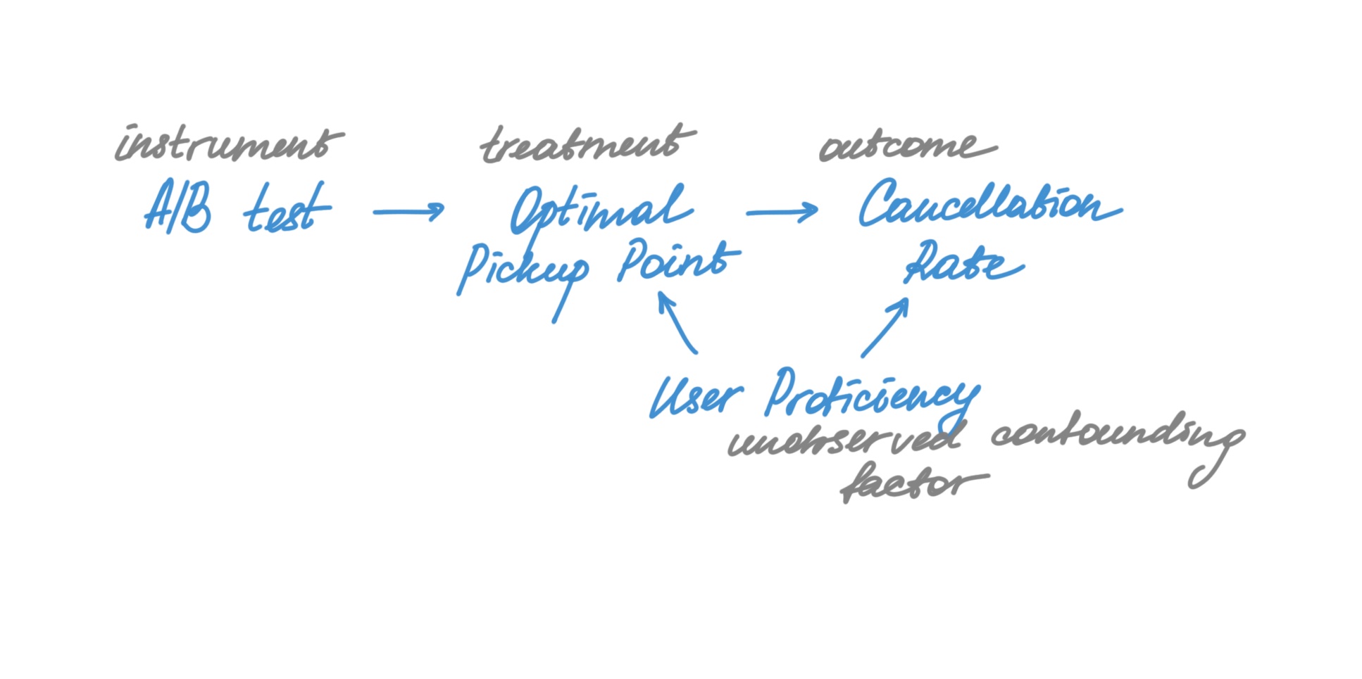
Suppose we are developing a clustering algorithm to recommend optimal pickup points for customers. The hypothesis is that this would reduce cancellations as popular pickup points facilitate easy meetups between drivers and customers. Here feature adoption is endogenous – frequent users may be more likely to adopt new features. The A/B test design should ensure that confounding factors are uniformly distributed across both groups. However, the actual impact may still be diluted. Instrumental variables can help provide a more precise estimation of the effect size. In the first stage, we build a model to predict the share of trips from recommended pickup points based on treatment assignment (our IV). Then we make the second stage regression of the cancellations rate based on the prediction from the first model and look at the coefficient to estimate the effect size and the significance.
A/B tests can be tailored specifically for IV estimation, often called Randomized Encouragement Trials. Such trials are handy when we want to nudge people towards a certain treatment but can’t make it happen directly. So you randomize the nudge, just like a normal AB test. For example, Twitch wanted to estimate how having more friends on the platform impacts a retention rate. We must be cautious about the assumption of exogeneity. Let’s say we nudge by email with suggestions to find and add some friends. If the control group received no email, this assumption isn’t valid: getting an email could drive retention. If the control group received an email similar to the test group but without mention of friends, the exclusion restriction likely holds.

Propensity Score Matching

This method finds its use when random assignment is not viable. It simulates a randomized experiment by ensuring comparability between treatment and control groups.

Assumptions

The key assumption is conditional independence or ignorability, meaning that given the propensity score, the distribution of observed outcomes in the treatment and control groups should be independent of the treatment assignment. It also requires that all relevant confounding variables be included in the propensity score model and there are no latent variables that affect treatment assignment. It also requires a large sample size for accurate matching.

Algorithm

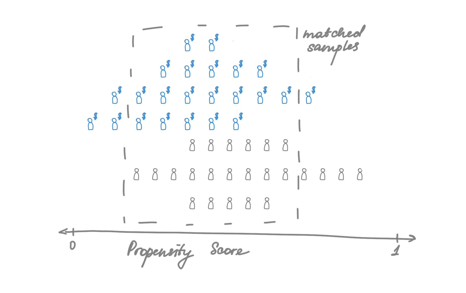
You estimate the probability of treatment assignment given a set of features, say, through logistic regression. This model need not be highly accurate; its construction should aim to control confounding rather than predict treatment.
For each treated unit, an untreated unit with a similar propensity for treatment is found. This can be done using Nearest Neighbor matching.
The average treatment effect is computed as the average outcome difference between the matched pairs.

For the simplest model, Scikit-Learn will do the job.

Examples

Suppose a company wants to evaluate the effectiveness of a new incentive program for drivers, which was not randomly rolled out. They can use PSM to match drivers who received the incentive with similar drivers who did not, based on variables like driving hours, number of rides completed, location, acceptance rate, etc. Then we can compare outcomes of interest between the two groups to estimate the effect of the incentive program.
There is also an interesting use case from Lyft where they run an A/B test on hardware splitting by bike units but also want to estimate the impact on users. So, they run two consecutive experiments, one real hardware-split test and one synthetic user-split test. Their synthetic test matches users who saw different variants to similar users who only saw the control via propensity score modeling. More details here.

Difference-in-Differences

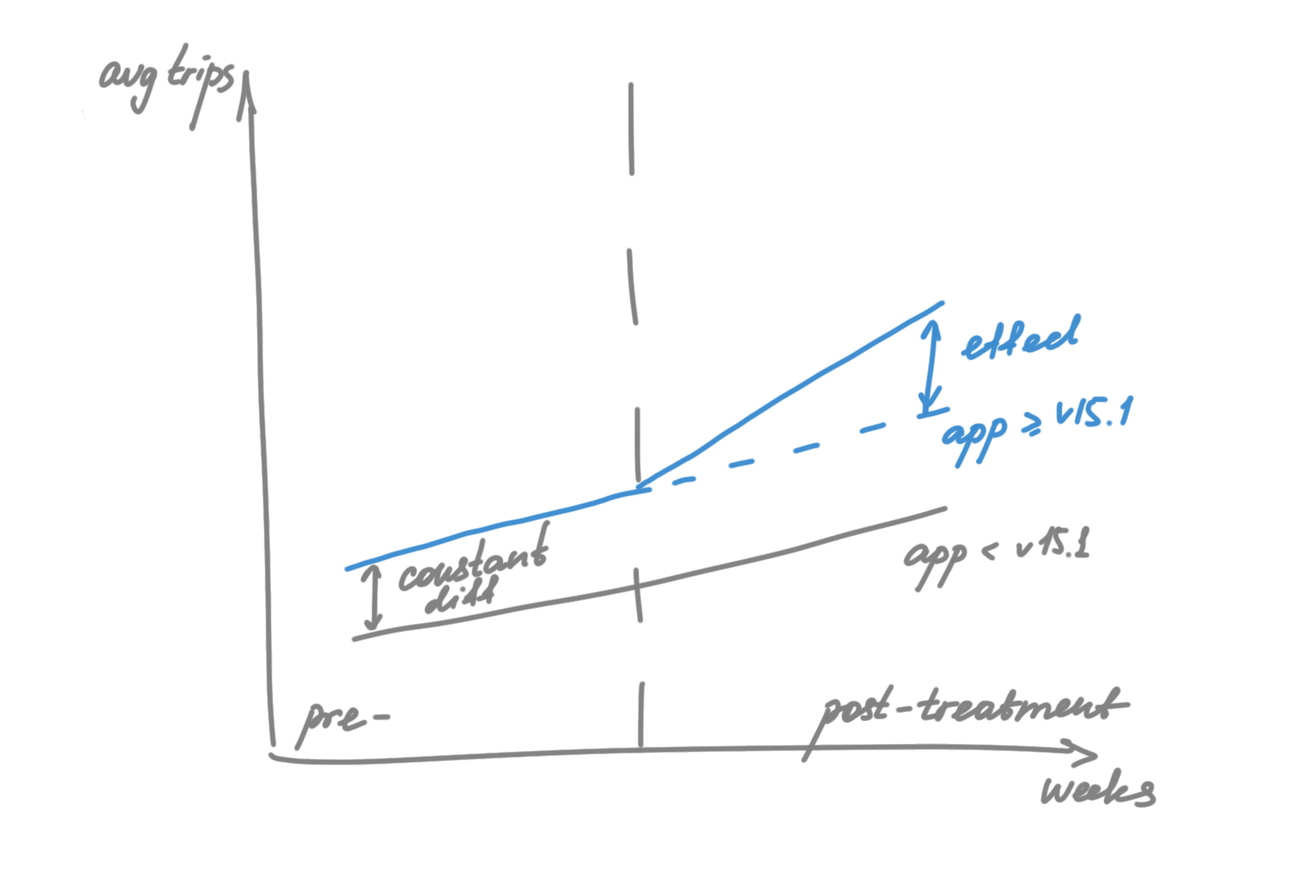
DiD is often the go-to when randomized experiments are unfeasible, unethical, or too costly. Data is collected pre and post-treatment from both the treated and control groups. The method calculates the effect of the treatment as the difference in the average change in outcome over time between these groups.

Assumptions

The DiD method rests on the parallel trends assumption. Without treatment, the average outcomes for the treated and control groups would have followed the same trend over time. Another crucial assumption is that exposure is exogenous and other factors that might be related to the outcome don’t influence the treatment assignment.

Algorithm

Identify your treatment and control groups and the periods before and after the treatment is applied, with the outcome that you are interested in. Inspect pre-treatment trends for the treated and control groups to check if they are parallel.
The simplest way to implement DiD is with a linear regression model, where the dependent variable is the outcome of interest. You include a binary variable for treatment (which is 1 for the treatment group and 0 for the control group), a binary variable for time (which is 1 for the time periods after treatment and 0 for the time periods before treatment), and a term for the interaction between treatment and time.
The coefficient on the interaction term with its significance is the DiD estimator of the treatment effect.

Examples

Let’s say we are launching a widget promoting COVID vaccination centers and want to estimate its impact on our business. It would be unethical to launch it just on the city’s share, plus we want to do a proper marketing campaign around that. So A/B is not an option. We launched the widget without randomized split, but it required an app update for the widget to be visible. So, we compared treatment (users with an updated app version) with control (others with an old version) with DiD. To mitigate the possible bias, we removed heavy users’ intentional app updates. More details here.
Another use case could be pricing changes. Ride-hailing industry has a network effect when drivers are shared between groups, so SUTVA can’t be guaranteed, and we can’t run an A/B experiment inside one city. So, we can use DiD to estimate the effect by selecting a market with parallel trends by key metrics with our target city and use it as control.

Want to dive deeper?

So, each method has its assumptions and is best suited to different scenarios. As with all statistical methods, it’s crucial to understand these assumptions and carefully check whether they hold in your particular situation. In practice, it’s often beneficial to use multiple methods and see if they provide consistent results, which can increase confidence in your findings.

The methods presented in the article are pretty basic and have more advantaged versions, so it’s worth exploring them further. The field of causal inference is relatively new and evolving quite fast. You can follow the progress through conferences like KDD and CLeaR.

There are also great resources to dive deeper into applications of CausalML:

Go home